Predicting House Prices: My Data Science Journey

Welcome to another blog post! Today, I’m delving into the exciting world of predictive modeling in real estate using the House Prices dataset from Kaggle’s Advanced Regression Techniques competition.
In this (brief) post, I’ll walk you through the entire process of preprocessing the data, building a machine learning model, and making predictions. So, grab your favorite beverage, and let’s dive in!

Introduction

The housing market is a complex ecosystem influenced by various factors ranging from location and size to architectural style and amenities. Predicting house prices accurately is crucial for both buyers and sellers. In this project, I aim to develop a robust predictive model that can estimate house prices based on several features provided in the dataset.

Exploring the Housing Dataset

Before diving into the pre-processing part, let’s first take a closer look at our dataset.
I started by conducting some general (statistical) checks using:

– the describe() function

– the info() function

- shape method

That gave me some knowledge about the summary statistics of the features (columns) and some key metrics like min/max values, and standard deviation of each column.

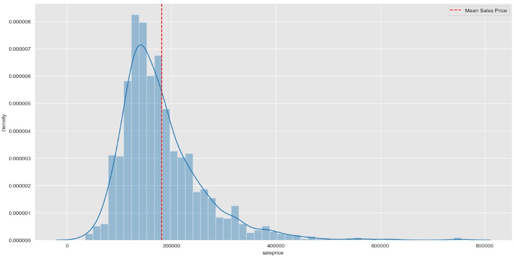
In order to gain more insights into the distribution of the sales prices I created a distribution plot that looks like this:

The distribution of the Sales Prices looks to be right skewed. This means:

• The Majority of Houses are Lower Priced: The peak of the distribution, where most of the data points lie, is towards the lower end of the price range. This suggests that there are more houses with lower prices compared to higher prices.

• Fewer Expensive Houses: As the distribution extends towards the higher prices, there are fewer houses with expensive prices. This could indicate that high-priced houses are less common or less frequently sold compared to lower-priced ones.

• Right Tail: The right-skewed nature of the distribution means that there are some houses with exceptionally high prices, leading to a longer tail on the right side of the distribution.

Preprocessing of the Data

Preprocessing of data is a vital step in every Data Science project. Most datasets are far from perfect and need to undergo vital steps for it to serve as input to a Machine Learning Model.

The steps I took in this housing dataset were:

1. Handling Missing Values

One of the initial challenges in any data science project is dealing with missing values. In my case most missing values existed in the ‘LotFrontage’ feature. In order to tackle this problem I created a Random Forest ML model to predict the values of this missing data. It would have been an option to remove this column from the dataset, or to remove rows with missing data, but I decided to pursue a more solid solution.

2. Checking for Outliers

Outliers can significantly impact the performance of predictive models. I utilized pairplots (see further) and the Z-score analysis to identify and remove outliers from the training data, ensuring the model learns from clean and reliable data.

3. Encoding Cat. Variables

Categorical variables need to be encoded into a numerical format before feeding them into machine learning models. I employed LabelEncoding to do so. LabelEncoding creates new columns where the categorial data is transformed into numbers.

Exploratory Data Analysis

Understanding Feature Relationships

Before getting into the model building, it’s essential to explore the relationships between our features and the target variable (Sales Price). I visualized these relationships using pairplots for both numeric and categorical features. This provides insights into potential correlations and trends.

In the 2 images below you can see the relationship between some numeric features and price (first one). The second one shows the count of categorical features.

Correlation Analysis

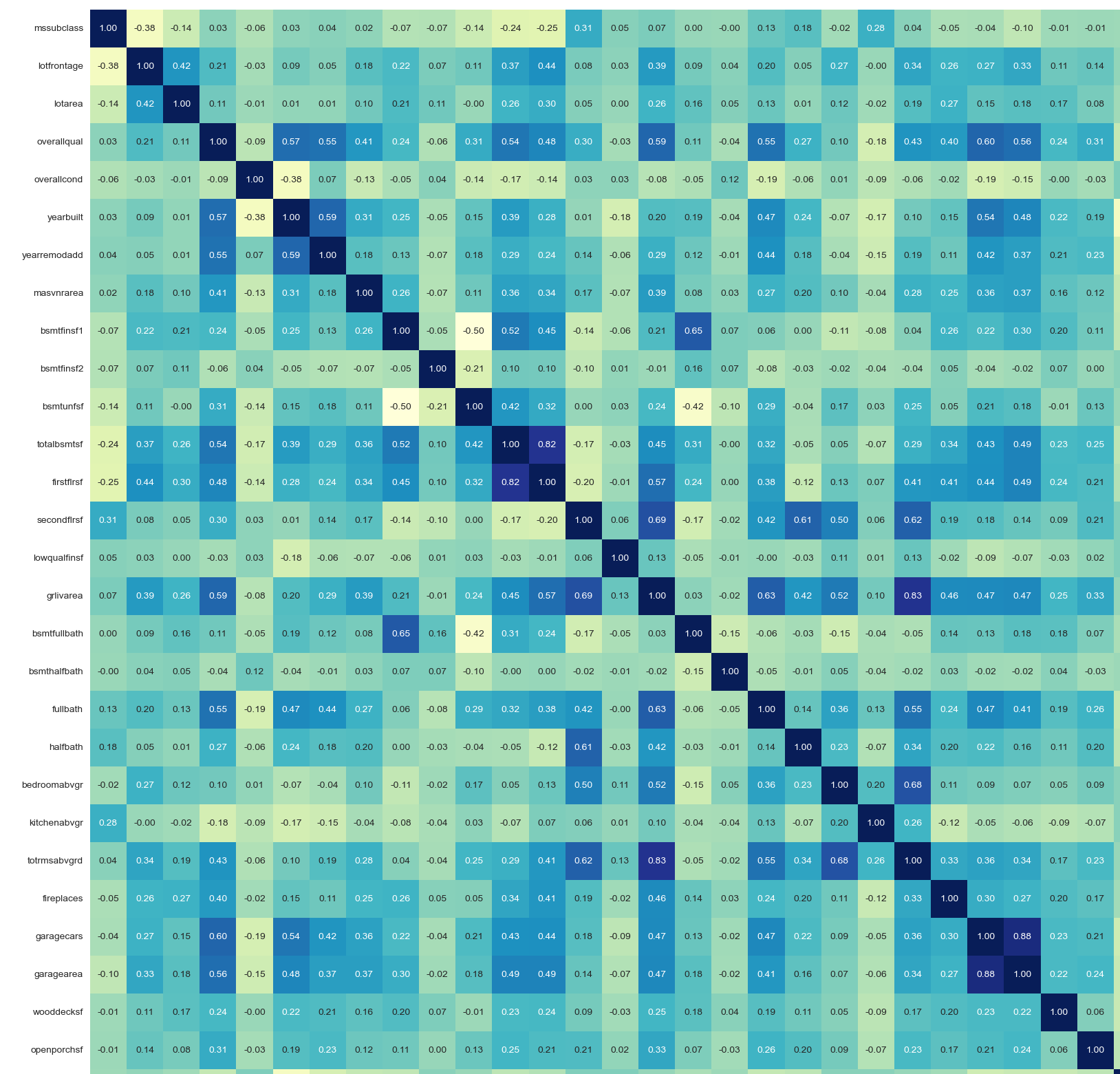
I calculated the correlation coefficients between numeric features and Sales Price and visualized them using a heatmap. This allowed us to identify the most influential features affecting house prices.

Building the Machine Learning Model

After completing the pre-processing steps, it is time to create the Machine Learning model. We are dealing with a challenge where we want to predict housing prices. As housing prices can take pretty much any value, we consider our predictions to be ‘continuous’ (as opposed to for example predicting a fixed outcome of ‘yes or no’, ‘true or false’ etc.).

Linear Regression

I started with a simple yet powerful Linear Regression model to predict the housing prices. After training the model on my pre-processed data, I evaluated its performance using metrics such as RMSE and R2 score.

In this first iteration the outcome was:

Validation score: 0.9244

Validation RMSE: 23816.8230

Test score: 0.8915

Test RMSE: 23576.6045

Interpretation:

• Overall, the linear regression model performs well on the test dataset, as indicated by the relatively high test score (0.8915) and the relatively low RMSE (23576.6045).
• The test score suggests that the model explains a large proportion of the variability in house prices using the available features.
• The RMSE indicates that, on average, the model’s predictions are approximately $23,576.60 away from the actual house prices in the test dataset.

Feature Importance

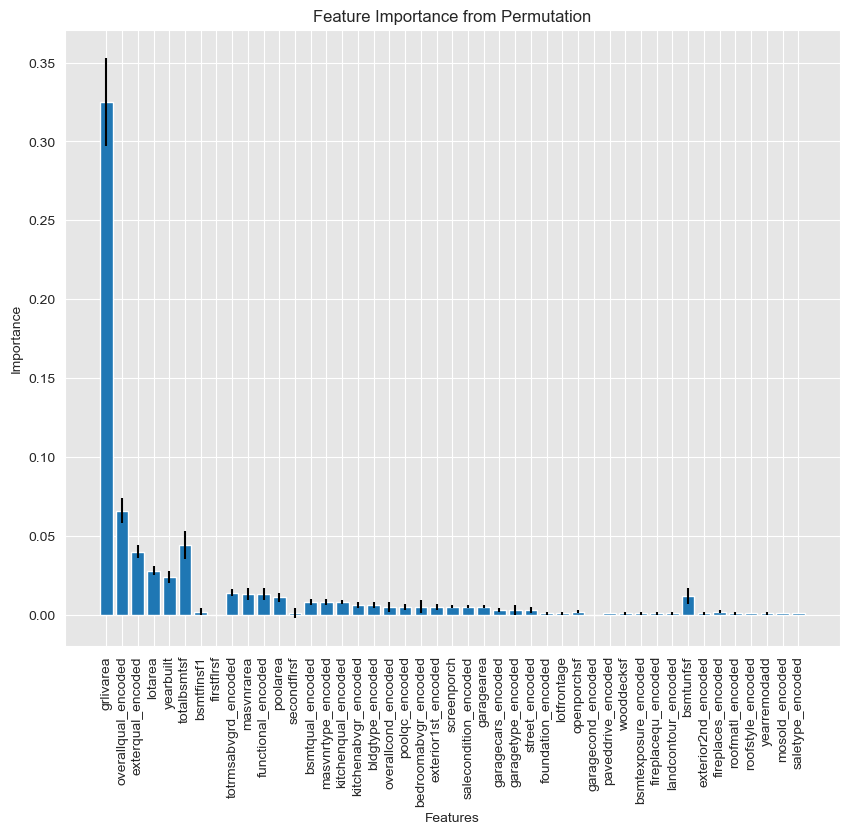
Understanding which features contribute the most to my model’s predictions is crucial for making informed decisions. I analysed feature importance using coefficients and permutation techniques, gaining insights into the key drivers of house prices.

The outcome of such analysis is depicted in the plot below. With this information I can take the most important features and neglect less importance features to improve the model even more.

This plot confirms the most important features (columns). Those are the size of the house, overall quality and the externals.

Model Evaluation and Prediction

Assessing Model Performance

I evaluated my model’s performance by comparing predicted values against actual values using scatter plots. This visual representation allowed me to identify areas of improvement and assess the model’s accuracy. I created a nice plot that instantly describes how well the model performs.

As you can see the model works pretty well and has a linear slope. There are a number of outliers, especially when prices are over 300k. The model seems to underestimate a number of cases. Further investigation, and maybe introducing a 2nd model for high-end homes, could improve my model’s accuracy.

Making Predictions

With the trained model, I’ve made predictions on the test dataset to participate in the Kaggle competition. I’m excited to see how my model performs against other competitors and contribute to the advancement of predictive modelling in real estate.

Stay tuned for updates on my model’s performance and further insights from the competition!

The entire code

Check out all of the code of this project at Github: Nick Analytics – House-Value-Prediction-with-ML